Heuristic Flow Control

Overview

The flexible services discussed in this article primarily refer to load balancing on the consumer side and rate limiting on the provider side. In previous versions of Dubbo,

• The load balancing component primarily focused on the principle of fairness, meaning that the consumer would choose from providers as equally as possible, which did not perform ideally in certain situations.
• The rate limiting component provided only static rate limiting schemes, requiring users to set static maximum concurrency values on the provider side, which are not easy for users to select reasonably.

We have made improvements to address these issues.

Load Balancing

Introduction

In the original version of Dubbo, there were five load balancing schemes to choose from: Random, ShortestResponse, RoundRobin, LeastActive, and ConsistentHash. Except for ShortestResponse and LeastActive, the other schemes mainly consider fairness and stability in selection.

For ShortestResponse, its design aims to select the provider with the shortest response time from all available options to improve overall system throughput. However, there are two issues:

1. In most scenarios, the response times of different providers do not show significant differences, causing the algorithm to degrade to random selection.
2. The length of the response time does not always represent the machine’s throughput capability. For LeastActive, it believes traffic should be allocated to machines currently handling fewer concurrent tasks, but it similarly faces issues like ShortestResponse, as it does not solely indicate the machine’s throughput capability.

Based on this analysis, we propose two new load balancing algorithms. One is a purely P2C algorithm based on fairness considerations, and the other is an adaptive method that attempts to measure the throughput capabilities of provider machines adaptively, allocating traffic to machines with higher throughput to enhance overall system performance.

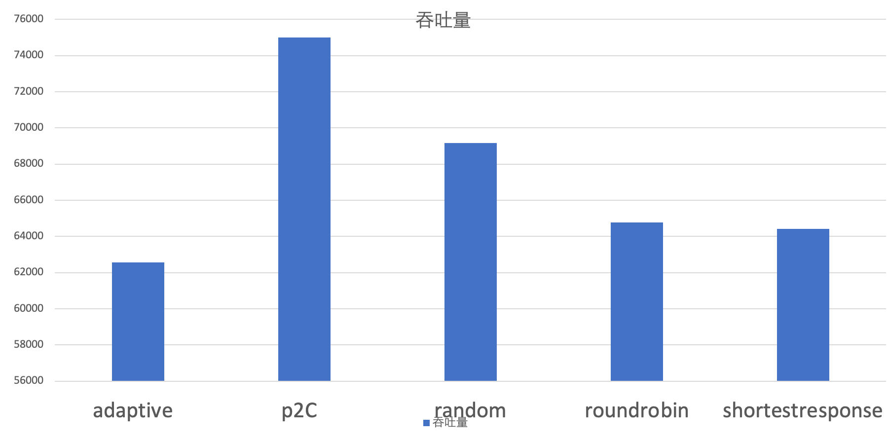
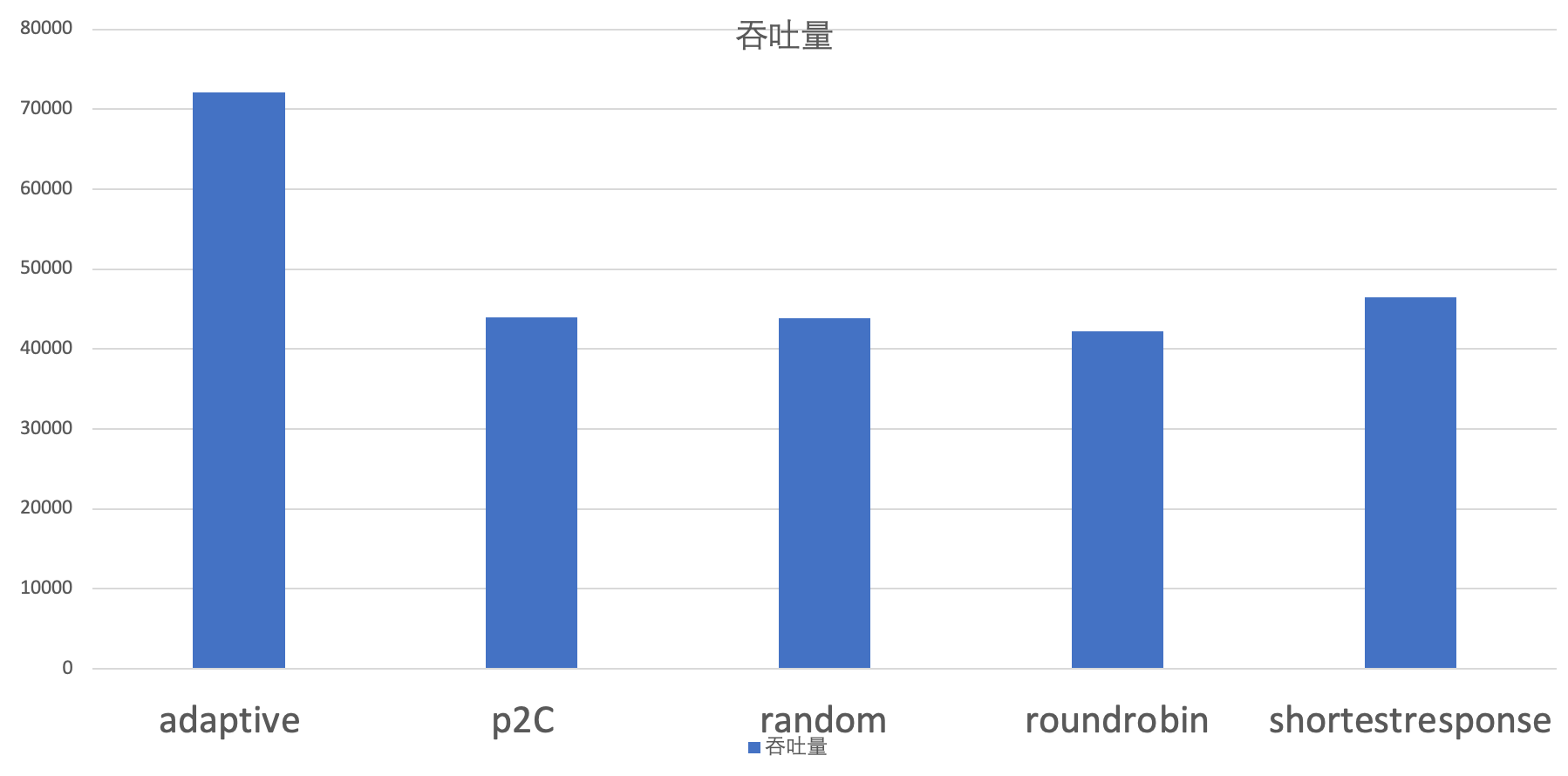
Overall Effect

The effectiveness experiments for load balancing were conducted in two different scenarios: one with relatively balanced provider configurations and another with significant disparities in provider configurations.

Usage Method

The usage method is the same as the original load balancing methods. Simply set “loadbalance” to “p2c” or “adaptive” on the consumer side.

Code Structure

The algorithm implementation for the load balancing part only requires inheriting the LoadBalance interface within the existing load balancing framework.

Principles

P2C Algorithm

The Power of Two Choices algorithm is simple yet classic, and its main idea is as follows:

1. For each call, make two random selections from the available provider list, choosing two nodes providerA and providerB.
2. Compare the two nodes, providerA and providerB, and select the one with the smaller “current number of connections being processed”.

Adaptive Algorithm

Code GitHub Link

Relevant Metrics

1. cpuLoad . This metric is obtained on the provider side and passed to the consumer side through the invocation’s attachments.

2. rt rt is the time taken for a single RPC call, measured in milliseconds.

3. timeout timeout is the remaining timeout for the current RPC call, measured in milliseconds.

4. weight weight is the configured service weight.

5. currentProviderTime The time at which the provider side calculates cpuLoad, measured in milliseconds.

6. currentTime currentTime is the last time load was calculated, initialized to currentProviderTime, measured in milliseconds.

7. multiple

8. lastLatency

9. beta Smoothing parameter, default is 0.5.

10. ewma The smoothed value of lastLatency

11. inflight inflight is the number of requests on the consumer side that have not yet been returned.

12. load For the alternate backend machine x, if the time since the last call is greater than 2*timeout, its load value is 0. Otherwise,

Algorithm Implementation

Still based on the P2C algorithm.

1. Randomly select two times from the alternative list to get providerA and providerB.
2. Compare the load values of providerA and providerB, choosing the smaller one.

Adaptive Rate Limiting

Unlike load balancing, which runs on the consumer side, the rate limiting feature operates on the provider side. Its purpose is to limit the maximum number of concurrent tasks processed by the provider. Theoretically, the server’s processing capacity has an upper limit. When a large number of request calls occur in a short period of time, it can lead to a backlog of unprocessed requests, overloading the machine. In such cases, two issues may arise: 1. Due to the request backlog, all requests must wait a long time to be processed, causing the entire service to go down. 2. Long-term overload of the server machine may risk crashing. Therefore, when there is potentially a risk of overload, rejecting some requests might be the better choice. In previous versions of Dubbo, rate limiting was implemented by setting a static maximum concurrency value on the provider side. However, in situations with numerous services and complex topology where processing capacity can dynamically change, it’s challenging for users to set this value statically. For these reasons, we need an adaptive algorithm that can dynamically adjust the maximum concurrency values of server machines, allowing them to process as many received requests as possible while ensuring the machines do not become overloaded. Therefore, we implemented two adaptive rate limiting algorithms within the Dubbo framework, based on heuristic smoothing: “HeuristicSmoothingFlowControl” and a window-based “AutoConcurrencyLimier”.

Code GitHub Link

Introduction

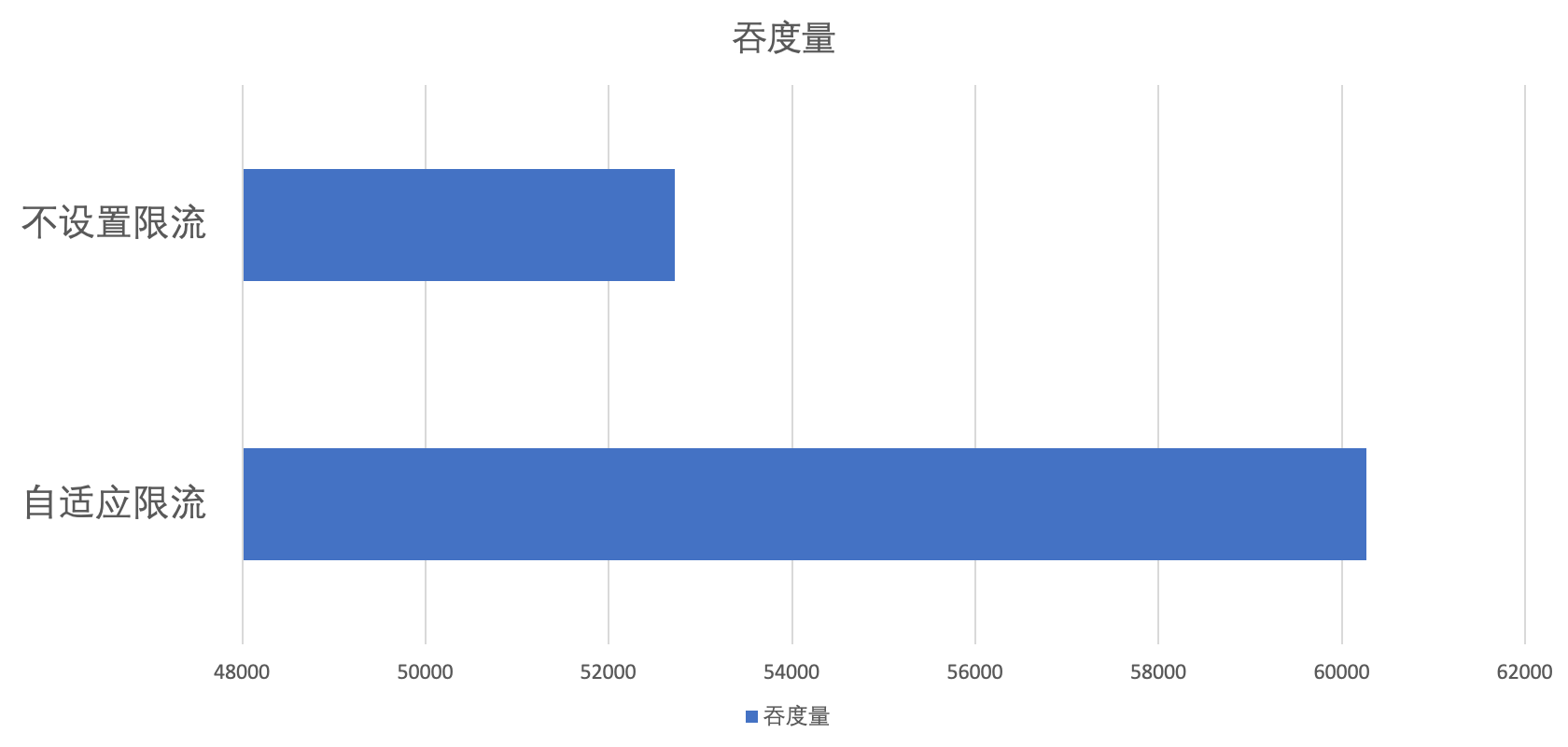
Overall Effect

The effectiveness experiments for adaptive rate limiting were conducted under the assumption of the provider’s machine configuration being as large as possible. To highlight the effects, we increased the complexity of single requests, set the timeout as large as possible, and enabled the retry feature on the consumer side.

Usage Method

To ensure that multiple nodes exist on the server side and that the retry strategy is enabled on the consumer side, the rate limiting function can perform better.

The configuration method is similar to setting the static maximum concurrency value; simply set “flowcontrol” to “autoConcurrencyLimier” or “heuristicSmoothingFlowControl” on the provider side.

Code Structure

1. FlowControlFilter: The filter on the provider side responsible for implementing rate limiting based on the algorithm’s results.
2. FlowControl: The interface for rate limiting algorithms implemented based on Dubbo’s SPI. The specific implementation algorithm needs to inherit from this interface and can be used through Dubbo’s SPI.
3. CpuUsage: Periodically fetches CPU-related metrics.
4. HardwareMetricsCollector: Methods for obtaining hardware metrics.
5. ServerMetricsCollector: Methods for obtaining the metrics necessary for rate limiting based on sliding windows, such as QPS, etc.
6. AutoConcurrencyLimier: The specific implementation algorithm for adaptive rate limiting.
7. HeuristicSmoothingFlowControl: The specific implementation method for adaptive rate limiting.

Principles

HeuristicSmoothingFlowControl

Relevant Metrics

1. alpha alpha is the acceptable increase in delay, defaulting to 0.3.

2. minLatency The minimum Latency value within a time window.

3. noLoadLatency noLoadLatency is the latency for purely processing tasks, excluding queue time. This is an inherent property of the server machine, but not static. In the HeuristicSmoothingFlowControl algorithm, we determine the current noLoadLatency based on the CPU usage of the machine. When the CPU usage is low, we consider minLatency to be noLoadLatency. When CPU usage is moderate, we smoothly use minLatency to update the value of noLoadLatency. When CPU usage is high, the value of noLoadLatency does not change.

4. maxQPS The maximum QPS within a time window cycle.

5. avgLatency The average Latency within a time window cycle, measured in milliseconds.

6. maxConcurrency The current maximum concurrency value calculated for the service provider.

Algorithm Implementation

When the server receives a request, it first checks whether the CPU usage exceeds 50%. If it does not exceed 50%, the request is accepted for processing. If it exceeds 50%, it indicates that the current load is high, thus obtaining the current maxConcurrency value from the HeuristicSmoothingFlowControl algorithm. If the number of currently processing requests exceeds maxConcurrency, the request is rejected.

AutoConcurrencyLimier

Relevant Metrics

1. MaxExploreRatio Default set to 0.3.

2. MinExploreRatio Default set to 0.06.

3. SampleWindowSizeMs Length of the sampling window. Defaults to 1000 milliseconds.

4. MinSampleCount Minimum number of requests in the sampling window. Defaults to 40.

5. MaxSampleCount Maximum number of requests in the sampling window. Defaults to 500.

6. emaFactor Smoothing processing parameter. Defaults to 0.1.

7. exploreRatio Exploration rate. Initially set to MaxExploreRatio. If avgLatency <= noLoadLatency * (1.0 + MinExploreRatio) or qps >= maxQPS * (1.0 + MinExploreRatio), then exploreRatio = min(MaxExploreRatio, exploreRatio + 0.02). Otherwise, exploreRatio = max(MinExploreRatio, exploreRatio - 0.02).

8. maxQPS The maximum QPS within the window cycle.

9. noLoadLatency

10. halfSampleIntervalMs Half sampling interval. Defaults to 25000 milliseconds.

11. resetLatencyUs The timestamp for the next reset of all values, including window values and noLoadLatency. Measured in microseconds. Initialized to 0.

12. remeasureStartUs The start time for the next reset of the window.

13. startSampleTimeUs The time to start sampling. Measured in microseconds.

14. sampleCount The number of requests within the current sampling window.

15. totalSampleUs The sum of latencies for all requests in the sampling window. Measured in microseconds.

16. totalReqCount The total number of requests within the sampling window. Note the distinction from sampleCount.

17. samplingTimeUs The timestamp for the current request sampling. Measured in microseconds.

18. latency The latency for the current request.

19. qps The QPS value within that time window.

20. avgLatency The average latency within the window.

21. maxConcurrency The maximum concurrency value for the current cycle calculated from the previous window.

22. nextMaxConcurrency The next maximum concurrency value calculated for the current window.

Little’s Law

• When the service is in a stable state: concurrency = latency * qps. This is the basis for adaptive rate limiting theory.
• When requests do not cause the machine to be overloaded, latency is generally stable, and qps and concurrency exhibit a linear relationship.
• When the number of requests exceeds limits within a short time, causing the service to overload, both concurrency and latency will rise, and qps will tend to stabilize.

Algorithm Implementation

The algorithm use process of AutoConcurrencyLimier is similar to HeuristicSmoothingFlowControl. The major difference from HeuristicSmoothingFlowControl is that:

AutoConcurrencyLimier is window-based. Only when a certain amount of sampling data is accumulated within the window does it use the data to update maxConcurrency. Additionally, it uses exploreRatio to explore the remaining capacity.

Furthermore, every once in a while, max_concurrency will automatically be reduced and maintained for some time to address situations where noLoadLatency rises. This is difficult to avoid because estimating noLoadLatency requires the service to be at a low load state.

Since max_concurrency < concurrency, the service will reject all requests and set the “waiting time for all queued requests” in the rate limiting algorithm to 2 * latency, ensuring the majority of the minLatency samples have not undergone queuing.

• ←Previous
• Next→